70B Quality at 1.1B: What Booking.com's Best-Paper Pipeline Actually Did
💡 Tool Tip: AI Token Counter, Response Time Calculator, AI ROI Calculator
On October 30, 2026, Amazon Science published the full production write-up behind a paper that won the ACL 2025 Industry Track best-paper award, chosen from 421 submissions. The title is "Speed Without Sacrifice," and the method is almost disappointingly plain: distil Llama-3.1 at 70 billion parameters into a 1.1-billion-parameter TinyLlama, bolt on Medusa speculative decoding heads, and end up matching the teacher's quality while running 10 to 20 times faster at under a third of the cost of comparable open models. Three features, all on live Booking.com traffic, all validated with real users rather than offline similarity scores.

Distillation cuts the cost of each pass; Medusa cuts how many passes you need. The two dimensions multiply.
1. The constraint that started it
Booking.com answers tens of millions of queries a day. AI Trip Planner has to pull travel preferences out of a conversation in under a second. Smart Filters turns a sentence of natural language into structured filters in real time. Accommodation description generation produces copy across millions of listings. In all three the model was good enough and the unit economics were not. The industry's standard answer is binary — serve something smaller and eat the quality loss, or serve the big model and pay for it. This team went looking for a third option: shrink the model, then get more tokens out of every pass.
2. Why the two techniques multiply rather than add
Standard autoregressive decoding is memory-bandwidth bound, not compute bound: every generated token requires one full forward pass over the weights. Knowledge distillation attacks how expensive each pass is, because a smaller model means a cheaper step. Medusa attacks how many passes you need, by predicting several tokens in parallel and verifying them in one go — accepted tokens are kept, rejected ones are discarded. Compress both dimensions and the gains compound approximately multiplicatively. That is the paper's most portable insight: do not ask which technique is better, ask which dimension is your bottleneck. If you are queue-bound, shrinking the model buys you little. If you are weight-read bound, stacking heads buys you nothing.
# Step 1: build the distillation corpus from unlabelled production text.
# The teacher's cost is a one-off; the student's cost is every request forever.
import json

def label_with_teacher(prompts, teacher, out_path="distill.jsonl"):
    kept = 0
    with open(out_path, "w") as fh:
        for p in prompts:
            r = teacher.generate(p, temperature=0.7, max_tokens=512)
            if not r.text.strip():
                continue  # an empty teacher answer teaches nothing
            fh.write(json.dumps({"prompt": p, "completion": r.text}) + "
")
            kept += 1
    print(f"teacher labelled {kept} examples")

# Keep this step boring and reproducible: same prompt set, same sampling
# settings, versioned output file. Your student inherits every mistake here.
3. Four experiments, with the numbers shown
Round one: fine-tune TinyLlama on task data only. It already beat few-shot GPT-4o, which is a useful reminder that domain tuning compensates for size — and it still fell short of the 70B teacher. Round two: add knowledge distillation, training the student on a blend of human-annotated and teacher-annotated data. That closed more than 90% of the student-teacher gap and made inference roughly six times faster. Round three: attach Medusa heads, which added a further 2 to 3.6 times on top of the six. Round four: train both in a single pipeline, ending at teacher-level quality and 10 to 20 times the speed depending on the use case. Note the six: it is not "small models are automatically 6x faster," it is a measured result for this task at this size ratio.
# Step 2: Medusa heads. Base weights frozen; each head predicts a token
# further ahead. Medusa-2 trains base and heads in one stage, which is why the
# authors preferred it for teams already juggling several production models.
import torch.nn as nn

class MedusaHead(nn.Module):
    def __init__(self, hidden: int = 2048, vocab: int = 32000):
        super().__init__()
        self.layers = nn.Sequential(
            nn.Linear(hidden, hidden),
            nn.SiLU(),
            nn.Linear(hidden, vocab),
        )

def build_heads(base, k: int = 4):
    for p in base.parameters():
        p.requires_grad_(False)      # freeze the distilled student
    return nn.ModuleList([MedusaHead() for _ in range(k)])

# At position t, head i is trained against token t+i+1. At inference you run
# the base once, verify the drafted tokens, and keep the longest accepted
# prefix. Speculation is cheap; verification is the bill.
4. Medusa-1 versus Medusa-2 is an operations decision
Both variants produced comparable speedups with no meaningful quality loss. Medusa-1 fine-tunes the base first, freezes it, then trains the heads separately. Medusa-2 trains everything in one stage. The authors picked Medusa-2, and the reason is not a score — it is the pipeline. One stage is simpler to run, and for a team already maintaining several production models, simpler is the whole argument. That is more reusable than any multiplier in the paper, because what you end up maintaining is not a result, it is a dozen small pipelines and the humans who babysit them.
# Step 3: speedup is not a constant, it is a function of acceptance rate.
# Measure it on your own traffic before you promise anyone "10x".
def tokens_per_pass(accept):
    """accept[i] = P(head i accepted | tokens 0..i-1 accepted)."""
    total, prod = 1.0, 1.0          # the base model always commits one token
    for a in accept:
        prod *= a
        total += prod
    return total

for rate in (0.9, 0.8, 0.7, 0.6):
    print(rate, round(tokens_per_pass([rate] * 4), 2))

# 4 heads at 0.9 acceptance ≈ 4.1 tokens per base forward pass.
# At 0.6 it collapses to ≈ 2.3. That gap is why the same technique gave 2x in
# one Booking.com feature and 3.6x in another — and it is an upper bound: the
# verification pass is not free.
5. What the three features actually bought
Smart Filters was the latency-critical one: responses 15 times faster for 99% of queries. AI Trip Planner gained 2.9% user engagement against GPT-3.5. Accommodation description generation produced 1.4% more "helpful" ratings at less than a third of GPT-4's cost. Read together, the three results are buying two different things — latency in the first two, cost in the third. The same pipeline, two very different payoffs. Before you copy it, decide which one you are actually buying, because the tuning that maximises acceptance rate is not always the tuning that minimises cost per thousand requests.
# Step 4: grade the student on the task metric, not on perplexity.
# Perplexity moving tells you the student is close. It does not tell you the
# feature got better.
import statistics

def evaluate(model, cases, metric):
    scores = []
    for c in cases:
        out = model.generate(c["prompt"], max_tokens=c.get("max_tokens", 256))
        scores.append(metric(out, c["expected"]))
    scores.sort()
    return {
        "n": len(scores),
        "mean": round(statistics.mean(scores), 3),
        "p10": round(scores[len(scores) // 10], 3),
    }

# Booking.com went further than offline metrics: the numbers that decided the
# rollout came from live A/B tests — engagement for the trip planner, and the
# share of "helpful" votes on generated accommodation descriptions.
6. The order of operations, if you are copying this
Measure a baseline first: p50, p95, cost per thousand requests, and one quality metric tied to the business instead of to the teacher. Then identify the bottleneck dimension — weight bandwidth or serial steps. Then distil, labelling unlabelled production text with the teacher, and accept that this step costs money once. Then attach heads and instrument acceptance rate as a first-class metric, because the speedup is almost entirely a function of it. Finally, decide on live A/B results rather than offline similarity. The failure mode here is a team that ships a 6x-slower-to-build pipeline and never measures the acceptance rate, then concludes distillation does not work.
# Step 5: cost per thousand requests, then the break-even.
def cost_per_1k(tokens_in, tokens_out, in_price, out_price, requests=1000):
    return requests * (tokens_in * in_price + tokens_out * out_price) / 1_000_000

teacher = cost_per_1k(600, 220, 2.50, 10.00)
student = cost_per_1k(600, 220, 0.05, 0.15)
print("teacher", round(teacher, 2), "vs student", round(student, 2), "per 1k requests")
print("ratio", round(teacher / student), "x cheaper")

# Then add the one-off: teacher labelling + GPU hours, divided by monthly
# request volume. If the break-even lands past the feature's expected life,
# the honest answer is that you should not build it yet.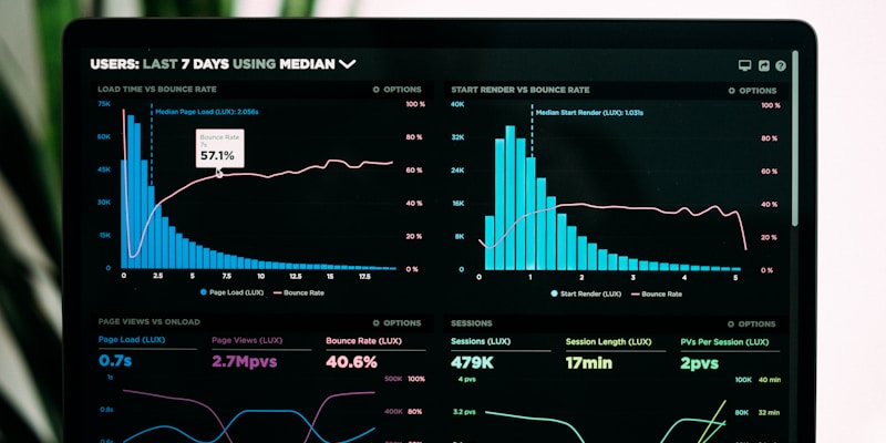
The same technique gave 2x on one feature and 3.6x on another. Acceptance rate explains the gap.
📌 Frequently Asked Questions
Can I apply the 20x speedup directly to my workload?
No. The paper reports 10 to 20 times depending on the use case, and the multiplier is driven mostly by speculative acceptance rate, which depends on how predictable your outputs are. Structured output and templated copy accept well; open-ended writing does not. Measure acceptance on your own traffic and derive the speedup instead of borrowing one.
Does distillation copy the teacher's flaws?
Yes. The student is trained on the teacher's outputs, so its preferences, formatting habits and mistakes are inherited. That is why the evaluation here included live metrics — engagement and helpfulness votes — and not only similarity to the teacher. If you copy the pipeline, add human spot checks to the offline stage at minimum.
Can a 1.1B student replace the 70B teacher for everything?
The paper scopes itself to three well-defined travel tasks, not general capability. Distillation compresses ability onto a task distribution, and behaviour outside that distribution degrades noticeably. If your product needs broad open-domain competence, route instead: predictable traffic to the small model, the long tail to a large one.
Why did the authors prefer Medusa-2 if Medusa-1 scored as well?
Because the measured speedups were comparable with no meaningful quality loss, and Medusa-2 is single-stage training, which is a simpler pipeline. For teams maintaining multiple models, removing a stage and a weight-freezing step means fewer operational failures.
Is this new research, or an old paper revisited?
The paper won the ACL 2025 Industry Track best-paper award. AWS published the production case study on Amazon Science on October 30, 2026, with the experiment order, the multiplier at each stage, and the live result for each of the three features. For anyone working on inference cost, the case study is more useful than the paper body.
🔧 Recommended Tools
AI Token Counter
Price a teacher pass before you run millions of them
Response Time Calculator
Convert acceptance rate into user-visible latency
AI ROI Calculator
Find the break-even on distillation
Diff Checker
Compare student and teacher outputs line by line
Prompt Cache Calculator
Cache helps; smaller models help more
📚 Sources
- Amazon Science — Speeding up language models for travel applications (Oct 30, 2026)
- ACL Anthology — Speed Without Sacrifice: Fine-Tuning Language Models with Medusa and Knowledge Distillation in Travel Applications
- arXiv — Medusa: Simple LLM Inference Acceleration Framework with Multiple Decoding Heads
- arXiv — Distilling the Knowledge in a Neural Network (Hinton et al.)
- Tech Times — AWS and Booking.com win ACL best paper by making a 70B model run 20x faster