开源权重拿下 71.5% 的 token、只有 23% 的花费:读懂 AI Gateway 生产指数
💡 工具推荐: AI Token 计数器, JSON 格式化, CSV 转 JSON, 时间戳转换
Vercel 在 10 月 14 日发布了 2026 年 10 月的 AI Gateway 生产指数,标题本身就是一条分裂的事实:开源权重模型现在处理 71.5% 的网关 token,却只占 23% 的花费。同一份报告还说,9 月网关花费约为 12 月的 13 倍,而每 token 均价下降了 47%;近三分之一的付费团队在一个月内更换了主力模型厂商,报告称这是该指数有记录以来的最高值;9 月花在中国来源模型上的钱,近七成经由美国厂商。这些数字单拎出来都好引用,放在一起说的是一件更有用的事:选模型已经变成组合管理,而把它当组合管理的团队,账单不再给他们惊喜。
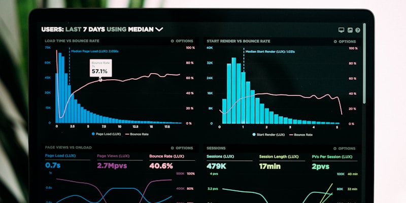
token 占比和花费占比天生就会分叉,那个缺口才是决策发生的地方。
两个占比,一个缺口
71.5% 和 23% 不矛盾,也不是文字游戏。它们是同一批流量的两个不同占比:某一类模型处理了多少 token,又吸走了多少美元。便宜的模型跑量,贵的模型干那些不能降级的工作。任何一个正常工作里的架构,这两个数字之间都会有缺口。
真正重要的是方向。开源权重的花费占比从 6 月的二十分之一,涨到 9 月的近四分之一。同一窗口里,前沿模型的花费涨了十倍,开源权重涨了七十多倍。增长率差到这个程度,说明变的是结构,不只是预算。
最容易犯的错是把它读成对质量的判决。它不是。它说的是边际 token 去了哪里:跑量的工作先下移到便宜档,因为那里的质量容差最宽,单位风险换来的节省最大。
# Before you have an opinion about the index, compute your own version of it.
# Two numbers per model: share of tokens, share of spend. They almost never match,
# and the gap is the whole story.

import json
from collections import defaultdict

rows = [json.loads(line) for line in open("gateway-usage.jsonl")]

tok = defaultdict(int)
spend = defaultdict(float)
for r in rows:
    m = r["model"]
    tok[m] += r["input_tokens"] + r["output_tokens"] + r.get("reasoning_tokens", 0)
    spend[m] += r["cost_usd"]

T, S = sum(tok.values()), sum(spend.values())
print(f"{'model':38} {'tok%':>7} {'spend%':>8} {'ratio':>7}")
for m in sorted(tok, key=lambda k: -tok[k]):
    t, s = 100 * tok[m] / T, 100 * spend[m] / S
    print(f"{m:38} {t:7.1f} {s:8.1f} {s / max(t, 1e-9):7.2f}")

# A ratio well above 1 means the model is expensive relative to how much you use it.
# A ratio near 0 means it is doing volume work and should never be your cost problem.
每 token 价格跌了 47%,你的账单却涨了
花上是 12 月的 13 倍,同时每 token 均价跌了 47%,这是报告里最不意外、也最常被误读的一句话。用量涨得比价格跌得快。这就是普及的样子,也正因为如此,只谈单价的成本治理往往会输。
标价还会以几种具体方式误导你的账单:没算进去的缓存命中、没进输出估算的推理 token、翻倍的重试请求,以及照样消耗输入但失败了的调用。只有从你自己日志里算出来的「每百万 token 有效价格」,才是能扛住账单检验的单位。
报告在这点上很谨慎:它写明花费是按公开标价估算、真实账单可能不同,token 口径包含输入、输出、推理、缓存输入和缓存创建。在预算会上引用任何百分比之前,先把这条脚注读完。
# Effective price per million tokens is the only comparable unit across models.
# Published rates lie about your bill in three ways: cache hits, reasoning tokens,
# and retries. Fold all of them into the same denominator.

def effective_price(calls):
    billable_in = sum(c.input_tokens for c in calls) - sum(c.cached_tokens for c in calls)
    billable_out = sum(c.output_tokens + c.reasoning_tokens for c in calls)
    cost = sum(c.cost_usd for c in calls)
    total = billable_in + billable_out
    return {
        "cost": round(cost, 2),
        "m_tokens": round(total / 1e6, 2),
        "usd_per_mtok": round(cost / max(total / 1e6, 1e-9), 3),
        "cache_hit_rate": round(sum(c.cached_tokens for c in calls) / max(billable_in, 1), 3),
    }

# Run this per model, per week. A model whose usd_per_mtok falls while its token
# share rises is being absorbed into the cheap tier of your architecture, which is
# exactly what the index describes happening across the whole gateway.
近三分之一团队换了主力厂商
这是我会拿到采购团队面前的那个数字。一个月里有三分之一的付费团队更换主力厂商,这不是品牌流失,这是切换成本崩掉的证据。报告还提到,期间流量在 1000 万 token 以上的团队平均用了 15 个模型,1 亿以上是 26 个,10 亿以上是 42 个。
把它当架构的规模规律来读,而不是购物习惯。流量越大,你能负担独立路由的切片越多,因为每个切片都测得清楚。多样化是在你拥有足够数据评估第二个选项之后自然长出来的。
实际推论是:路由策略应该是一个带版本号的产物。如果它只活在某个人脑子里,一次模型下线就是事故,而不是一次 diff。下面的策略故意写得很笨:档位、规则、升级路径,全都是数据。
# Routing is a portfolio decision, not a favourite-model decision. Write the policy
# down as data so it can be reviewed, diffed, and rolled back like code.

POLICY = {
    "tiers": {
        "cheap":    {"max_in_per_mtok": 0.30, "models": ["open-weight-fast-a", "open-weight-fast-b"]},
        "balanced": {"max_in_per_mtok": 2.00, "models": ["mid-a", "mid-b"]},
        "frontier": {"max_in_per_mtok": 12.0, "models": ["flagship-a", "flagship-b"]},
    },
    "rules": [
        {"when": "task == 'classification'", "tier": "cheap"},
        {"when": "task == 'code_edit' and files_changed <= 2", "tier": "balanced"},
        {"when": "task == 'migration_plan'", "tier": "frontier"},
    ],
    "on_failure": {"retry_same_tier": 1, "then": "escalate_one_tier"},
}

def pick(task, files_changed=0):
    for r in POLICY["rules"]:
        if eval(r["when"], {"__builtins__": {}}, {"task": task, "files_changed": files_changed}):
            return POLICY["tiers"][r["tier"]]["models"]
    return POLICY["tiers"]["balanced"]["models"]

# Rule of thumb from the index: cost control comes from moving volume down a tier,
# never from switching the flagship. Switching the flagship moves 3% of your bill.
print(pick("classification"), pick("migration_plan"))

按标价算的花费只是估算,唯一算数的是你的账单。
钱到底挪到了哪
报告里几个具体的数字值得当校准用。DeepSeek 的模型处理了全部网关 token 的 58%,只占 6.6% 的花费;单 DeepSeek-v4.1-Flash 就扛了 9 月近一半的 token,花掉 2.6% 的钱,单价约为开源权重均价的五分之一;Kimi K3 贡献了开源权重花费增量的近一半,而它处理的 token 少得多。
闭源这边,Anthropic 的网关花费占比从 63.7% 掉到 43.9%,首次跌破一半,其中 Opus 贡献了约 20 个点里的 17 个。Jev 在头两周触达 35% 的付费团队,是该指数历史上最快的采用速度,但那两周只占 0.27% 的网关花费。Opus 5.5 在头两周就拿走了超过十分之一的网关美元。
该记住的模式是:采用占比和花费占比是两个不同指标,而且往往指向相反方向。一个模型可以无处不在却几乎不花钱,也可以只有少数团队在用却扛着账单。评估一个新模型发布,用跟你工作负载匹配的那个指标,别用标题里的那个。
# Concentration check: how dependent are you on one lab? The index reports that
# teams above 10M tokens used an average of 15 models, 26 above 100M, and 42 above
# a billion. Volume forces diversification; policy should not lag behind volume.

from collections import Counter

def concentration(rows, by="lab"):
    spend = Counter()
    for r in rows:
        spend[r[by]] += r["cost_usd"]
    total = sum(spend.values()) or 1
    shares = [v / total for v in spend.values()]
    hhi = sum(s * s for s in shares)          # 1.0 = single vendor, lower = diversified
    return {
        "labs": len(spend),
        "top_share": round(max(shares), 3),
        "hhi": round(hhi, 3),
        "verdict": "fragile" if hhi > 0.5 else "concentrated" if hhi > 0.25 else "diversified",
    }

# A high HHI is not automatically bad. It is bad when you cannot name the second
# option, its measured quality delta, and the swap cost. If you cannot, you have a
# single point of failure with a monthly invoice attached.
在照抄市场之前,先重放你自己的流量
大多数团队就是在这里踩坑的。他们看到开源权重拿下 71.5% 的 token,就把一大块流量切到更便宜的模型,三周后发现某个没人写测试的工作流上工具调用准确率掉了。报告描述的是总量,你的任务分布不等于总量。
站得住的做法是重放:拿上个月的真实流量,算出在拟议组合下会花多少钱,再配上你自己评测集上量出来的质量差。如果你没有评测集,那才是真正的卡点,而且它比选哪个模型大得多。
报告没有明说但已经摊开的一件事是:厂商之间争的不再是「不可替代」,而是「可被重新选择」。那就按这个来设计架构:厂商边界做薄,提示词可迁移,路由表进版本控制,让切换是「一个下午」的事,而不是「一个季度」。
# Replay last month's traffic against a proposed mix. Estimates only: list prices,
# no cache effects you have not measured, and no retry amplification.

def replay(traffic, mix):
    # traffic: {"cheap": tokens, "balanced": tokens, "frontier": tokens}
    # mix: {"cheap": price_per_mtok, ...}
    return {tier: round(tokens / 1e6 * mix[tier], 2) for tier, tokens in traffic.items()}

current = {"cheap": 4.1e9, "balanced": 900e6, "frontier": 120e6}
old_mix = {"cheap": 0.06, "balanced": 0.90, "frontier": 5.00}
new_mix = {"cheap": 0.05, "balanced": 0.85, "frontier": 5.00}

print("current", replay(current, old_mix))
print("proposed", replay(current, new_mix))
# Move a slice of 'balanced' into 'cheap' only after you have measured the quality
# delta on your own eval set. The index says the market did this at scale; it does
# not say your task tolerates it.

模型由谁托管,影响成本、延迟,现在也影响采购决策。
📌 常见问题 FAQ
71.5% 和 23% 到底在量什么?
它们是 2026 年 10 月报告里 AI Gateway 流量的两个占比:开源权重模型处理了 71.5% 的 token,占 23% 的花费。报告概括为「超过七成 token、近四分之一美元」。两者并不矛盾,因为便宜模型扛量、昂贵模型扛那些不能降级的工作。
报告里的花费是怎么算的?
报告写明:花费按公开标价估算,真实账单可能不同;每 token 均价等于估算花费除以 token 量。token 口径包含输入、输出、推理、缓存输入和缓存创建。
这是否说明开源权重模型什么都能干了?
不能这么说。指数衡量的是流量和钱去了哪里,不是质量对某个任务是否足够。把量迁到便宜模型,前提是你在自己的评测集上、按工作流量过质量差。
为什么流量越大,团队用的模型越多?
报告提到,期间 1000 万 token 以上的团队平均用了 15 个模型,1 亿以上 26 个,10 亿以上 42 个。流量越大,可分离的工作负载越多,而每个可分离负载都能独立路由和独立评测。
周一我该拿这份报告做什么?
从你自己的日志算出每个模型的 token 占比和花费占比,算出含缓存命中和推理 token 的「每百万 token 有效价格」,再看你对单一厂商的集中度。然后决定路由策略要不要写成代码。这是两小时的活,比再来一轮模型横评有用。